In physics, a gauge theory is a type of field theory in which the Lagrangian is invariant under acontinuous group of local transformations.
The term gauge refers to redundant degrees of freedom in the Lagrangian. The transformations between possible gauges, called gauge transformations, form a Lie group which is referred to as thesymmetry group or the gauge group of the theory. Associated with any Lie group is the Lie algebraof group generators. For each group generator there necessarily arises a corresponding vector fieldcalled the gauge field. Gauge fields are included in the Lagrangian to ensure its invariance under the local group transformations (called gauge invariance). When such a theory is quantized, the quantaof the gauge fields are called gauge bosons. If the symmetry group is non-commutative, the gauge theory is referred to as non-abelian, the usual example being the Yang–Mills theory.
Gauge theories are important as the successful field theories explaining the dynamics of elementary particles. Quantum electrodynamics is an abelian gauge theory with the symmetry group U(1) and has one gauge field, the electromagnetic field, with the photon being the gauge boson. The Standard Model is a non-abelian gauge theory with the symmetry group U(1)×SU(2)×SU(3) and has a total of twelve gauge bosons: the photon, three weak bosons and eight gluons.
Many powerful theories in physics are described by Lagrangians which are invariant under some symmetry transformation groups. When they are invariant under a transformation identically performed at every point in the space in which the physical processes occur, they are said to have aglobal symmetry. The requirement of local symmetry, the cornerstone of gauge theories, is a stricter constraint. In fact, a global symmetry is just a local symmetry whose group's parameters are fixed in space-time. Gauge symmetries can be viewed as analogues of the equivalence principle of general relativity in which each point in space-time is allowed a choice of local reference (coordinate) frame. Both symmetries reflect a redundancy in the description of a system.
Historically, these ideas were first stated in the context of classical electromagnetism and later ingeneral relativity. However, the modern importance of gauge symmetries appeared first in therelativistic quantum mechanics of electrons – quantum electrodynamics, elaborated on below. Today, gauge theories are useful in condensed matter, nuclear and high energy physics among other subfields.
[edit]History and importance
The earliest field theory having a gauge symmetry was Maxwell's formulation of electrodynamics in 1864. The importance of this symmetry remained unnoticed in the earliest formulations. Similarly unnoticed, Hilbert had derived the Einstein field equations by postulating the invariance of the actionunder a general coordinate transformation. Later Hermann Weyl, in an attempt to unify general relativity and electromagnetism, conjectured (incorrectly, as it turned out) that Eichinvarianz or invariance under the change of scale (or "gauge") might also be a local symmetry of general relativity. After the development of quantum mechanics, Weyl, Vladimir Fock and Fritz Londonmodified gauge by replacing the scale factor with a complex quantity and turned the scale transformation into a change of phase — a U(1) gauge symmetry. This explained theelectromagnetic field effect on the wave function of a charged quantum mechanical particle. This was the first widely recognised gauge theory, popularised by Pauli in the 1940s.[1]
In 1954, attempting to resolve some of the great confusion in elementary particle physics, Chen Ning Yang and Robert Mills introduced non-abelian gauge theories as models to understand the strong interaction holding together nucleons in atomic nuclei. (Ronald Shaw, working under Abdus Salam, independently introduced the same notion in his doctoral thesis.) Generalizing the gauge invariance of electromagnetism, they attempted to construct a theory based on the action of the (non-abelian) SU(2) symmetry group on the isospin doublet of protons and neutrons. This is similar to the action of the U(1) group on the spinor fields of quantum electrodynamics. In particle physics the emphasis was on using quantized gauge theories.
This idea later found application in the quantum field theory of the weak force, and its unification with electromagnetism in the electroweak theory. Gauge theories became even more attractive when it was realized that non-abelian gauge theories reproduced a feature called asymptotic freedom. Asymptotic freedom was believed to be an important characteristic of strong interactions. This motivated searching for a strong force gauge theory. This theory, now known as quantum chromodynamics, is a gauge theory with the action of the SU(3) group on the color triplet of quarks. The Standard Model unifies the description of electromagnetism, weak interactions and strong interactions in the language of gauge theory.
In the 1970s, Sir Michael Atiyah began studying the mathematics of solutions to the classical Yang–Mills equations. In 1983, Atiyah's student Simon Donaldson built on this work to show that thedifferentiable classification of smooth 4-manifolds is very different from their classification up tohomeomorphism. Michael Freedman used Donaldson's work to exhibit exotic R4s, that is, exoticdifferentiable structures on Euclidean 4-dimensional space. This led to an increasing interest in gauge theory for its own sake, independent of its successes in fundamental physics. In 1994,Edward Witten and Nathan Seiberg invented gauge-theoretic techniques based on supersymmetrywhich enabled the calculation of certain topological invariants. These contributions to mathematics from gauge theory have led to a renewed interest in this area.
The importance of gauge theories in physics is exemplified in the tremendous success of the mathematical formalism in providing a unified framework to describe the quantum field theories ofelectromagnetism, the weak force and the strong force. This theory, known as the Standard Model, accurately describes experimental predictions regarding three of the four fundamental forces of nature, and is a gauge theory with the gauge group SU(3) × SU(2) × U(1). Modern theories like string theory, as well as some formulations of general relativity, are, in one way or another, gauge theories.
- See Pickering for more about the history of gauge and quantum field theories.[2]
[edit]Description
[edit]Global and local symmetries
In physics, the mathematical description of any physical situation usually contains excess degrees of freedom; the same physical situation is equally well described by many equivalent mathematical configurations. For instance, in Newtonian dynamics, if two configurations are related by a Galilean transformation—an inertial change of reference frame—they represent the same physical situation. These transformations form a group of "symmetries" of the theory, and a physical situation corresponds not to an individual mathematical configuration but to a class of configurations related to one another by this symmetry group. This idea can be generalized to include local as well as global symmetries, analogous to much more abstract "changes of coordinates" in a situation where there is no preferred "inertial" coordinate system that covers the entire physical system. A gauge theory is a mathematical model that has symmetries of this kind, together with a set of techniques for making physical predictions consistent with the symmetries of the model.
[edit]Example of global symmetry
When a quantity occurring in the mathematical configuration is not just a number but has some geometrical significance, such as a velocity or an axis of rotation, its representation as numbers arranged in a vector or matrix is also changed by a coordinate transformation. For instance, if one description of a pattern of fluid flow states that the fluid velocity in the neighborhood of (x=1, y=0) is 1 m/s in the positive x direction, then a description of the same situation in which the coordinate system has been rotated clockwise by 90 degrees will state that the fluid velocity in the neighborhood of (x=0, y=1) is 1 m/s in the positive y direction. The coordinate transformation has affected both the coordinate system used to identify the location of the measurement and the basis in which its valueis expressed. As long as this transformation is performed globally (affecting the coordinate basis in the same way at every point), the effect on values that represent the rate of change of some quantity along some path in space and time as it passes through point P is the same as the effect on values that are truly local to P.
[edit]Use of fiber bundles to describe local symmetries
In order to adequately describe physical situations in more complex theories, it is often necessary to introduce a "coordinate basis" for some of the objects of the theory that do not have this simple relationship to the coordinates used to label points in space and time. (In mathematical terms, the theory involves a fiber bundle in which the fiber at each point of the base space consists of possible coordinate bases for use when describing the values of objects at that point.) In order to spell out a mathematical configuration, one must choose a particular coordinate basis at each point (a local section of the fiber bundle) and express the values of the objects of the theory (usually "fields" in the physicist's sense) using this basis. Two such mathematical configurations are equivalent (describe the same physical situation) if they are related by a transformation of this abstract coordinate basis (a change of local section, or gauge transformation).
In most gauge theories, the set of possible transformations of the abstract gauge basis at an individual point in space and time is a finite-dimensional Lie group. The simplest such group is U(1), which appears in the modern formulation of quantum electrodynamics (QED) via its use of complex numbers. QED is generally regarded as the first, and simplest, physical gauge theory. The set of possible gauge transformations of the entire configuration of a given gauge theory also forms a group, the gauge group of the theory. An element of the gauge group can be parameterized by a smoothly varying function from the points of spacetime to the (finite-dimensional) Lie group, whose value at each point represents the action of the gauge transformation on the fiber over that point.
A gauge transformation with constant parameter at every point in space and time is analogous to a rigid rotation of the geometric coordinate system; it represents a global symmetry of the gauge representation. As in the case of a rigid rotation, this gauge transformation affects expressions that represent the rate of change along a path of some gauge-dependent quantity in the same way as those that represent a truly local quantity. A gauge transformation whose parameter is not a constant function is referred to as a local symmetry; its effect on expressions that involve a derivative is qualitatively different from that on expressions that don't. (This is analogous to a non-inertial change of reference frame, which can produce a Coriolis effect.)
[edit]Gauge fields
The "gauge covariant" version of a gauge theory accounts for this effect by introducing a gauge field(in mathematical language, an Ehresmann connection) and formulating all rates of change in terms of the covariant derivative with respect to this connection. The gauge field becomes an essential part of the description of a mathematical configuration. A configuration in which the gauge field can be eliminated by a gauge transformation has the property that its field strength (in mathematical language, its curvature) is zero everywhere; a gauge theory is not limited to these configurations. In other words, the distinguishing characteristic of a gauge theory is that the gauge field does not merely compensate for a poor choice of coordinate system; there is generally no gauge transformation that makes the gauge field vanish.
When analyzing the dynamics of a gauge theory, the gauge field must be treated as a dynamical variable, similarly to other objects in the description of a physical situation. In addition to itsinteraction with other objects via the covariant derivative, the gauge field typically contributes energyin the form of a "self-energy" term. One can obtain the equations for the gauge theory by:
- starting from a naïve ansatz without the gauge field (in which the derivatives appear in a "bare" form);
- listing those global symmetries of the theory that can be characterized by a continuous parameter (generally an abstract equivalent of a rotation angle);
- computing the correction terms that result from allowing the symmetry parameter to vary from place to place; and
- reinterpreting these correction terms as couplings to one or more gauge fields, and giving these fields appropriate self-energy terms and dynamical behavior.
This is the sense in which a gauge theory "extends" a global symmetry to a local symmetry, and closely resembles the historical development of the gauge theory of gravity known as general relativity.
[edit]Physical experiments
Gauge theories are used to model the results of physical experiments, essentially by:
- limiting the universe of possible configurations to those consistent with the information used to set up the experiment, and then
- computing the probability distribution of the possible outcomes that the experiment is designed to measure.
The mathematical descriptions of the "setup information" and the "possible measurement outcomes" (loosely speaking, the "boundary conditions" of the experiment) are generally not expressible without reference to a particular coordinate system, including a choice of gauge. (If nothing else, one assumes that the experiment has been adequately isolated from "external" influence, which is itself a gauge-dependent statement.) Mishandling gauge dependence in boundary conditions is a frequent source of anomalies in gauge theory calculations, and gauge theories can be broadly classified by their approaches to anomaly avoidance.
[edit]Continuum theories
The two gauge theories mentioned above (continuum electrodynamics and general relativity) are examples of continuum field theories. The techniques of calculation in a continuum theory implicitly assume that:
- given a completely fixed choice of gauge, the boundary conditions of an individual configuration can in principle be completely described;
- given a completely fixed gauge and a complete set of boundary conditions, the principle of least action determines a unique mathematical configuration (and therefore a unique physical situation) consistent with these bounds;
- the likelihood of possible measurement outcomes can be determined by:
- establishing a probability distribution over all physical situations determined by boundary conditions that are consistent with the setup information,
- establishing a probability distribution of measurement outcomes for each possible physical situation, and
- convolving these two probability distributions to get a distribution of possible measurement outcomes consistent with the setup information; and
- fixing the gauge introduces no anomalies in the calculation, due either to gauge dependence in describing partial information about boundary conditions or to incompleteness of the theory.
These assumptions are close enough to valid across a wide range of energy scales and experimental conditions, to allow these theories to make accurate predictions about almost all of the phenomena encountered in daily life, from light, heat, and electricity to eclipses and spaceflight. They fail only at the smallest and largest scales (due to omissions in the theories themselves) and when the mathematical techniques themselves break down (most notably in the case of turbulence and other chaotic phenomena).
[edit]Quantum field theories
Other than these "classical" continuum field theories, the most widely known gauge theories arequantum field theories, including quantum electrodynamics and the Standard Model of elementary particle physics. The starting point of a quantum field theory is much like that of its continuum analog: a gauge-covariant action integral which characterizes "allowable" physical situations according to theprinciple of least action. However, continuum and quantum theories differ significantly in how they handle the excess degrees of freedom represented by gauge transformations. Continuum theories, and most pedagogical treatments of the simplest quantum field theories, use a gauge fixingprescription to reduce the orbit of mathematical configurations that represent a given physical situation to a smaller orbit related by a smaller gauge group (the global symmetry group, or perhaps even the trivial group).
More sophisticated quantum field theories, in particular those which involve a non-abelian gauge group, break the gauge symmetry within the techniques of perturbation theory by introducing additional fields (the Faddeev–Popov ghosts) and counterterms motivated by anomaly cancellation, in an approach known as BRST quantization. While these concerns are in one sense highly technical, they are also closely related to the nature of measurement, the limits on knowledge of a physical situation, and the interactions between incompletely specified experimental conditions and incompletely understood physical theory. The mathematical techniques that have been developed in order to make gauge theories tractable have found many other applications, from solid-state physicsand crystallography to low-dimensional topology.
[edit]Classical gauge theory
[edit]Classical electromagnetism
Historically, the first example of gauge symmetry to be discovered was classical electromagnetism. In electrostatics, one can either discuss the electric field, E, or its corresponding electric potential, V. Knowledge of one makes it possible to find the other, except that potentials differing by a constant,  , correspond to the same electric field. This is because the electric field relates tochanges in the potential from one point in space to another, and the constant C would cancel out when subtracting to find the change in potential. In terms of vector calculus, the electric field is thegradient of the potential,
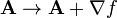
  . Generalizing from static electricity to electromagnetism, we have a second potential, the vector potential A, with


The general gauge transformations now become not just but
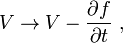
where f is any function that depends on position and time. The fields remain the same under the gauge transformation, and therefore Maxwell's equations are still satisfied. That is, Maxwell's equations have a gauge symmetry.
[edit]An example: Scalar O(n) gauge theory
- The remainder of this section requires some familiarity with classical or quantum field theory, and the use of Lagrangians.
- Definitions in this section: gauge group, gauge field, interaction Lagrangian, gauge boson.
The following illustrates how local gauge invariance can be "motivated" heuristically starting from global symmetry properties, and how it leads to an interaction between fields which were originally non-interacting.
Consider a set of n non-interacting scalar fields, with equal masses m. This system is described by an action which is the sum of the (usual) action for each scalar field 
![\mathcal{S} = \int \, \mathrm{d}^4 x \sum_{i=1}^n \left[ \frac{1}{2} \partial_\mu \varphi_i \partial^\mu \varphi_i - \frac{1}{2}m^2 \varphi_i^2 \right].](http://upload.wikimedia.org/wikipedia/en/math/e/2/0/e203919f483ea9b2a681a26e4292920b.png)
The Lagrangian (density) can be compactly written as
-
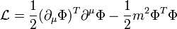
by introducing a vector of fields

The term  is Einstein notation for the partial derivative of
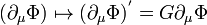
  in each of the four dimensions. It is now transparent that the Lagrangian is invariant under the transformation
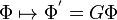
whenever G is a constant matrix belonging to the n-by-n orthogonal group O(n). This is seen to preserve the Lagrangian since the derivative of will transform identically to and both quantities appear inside dot products in the Lagrangian (orthogonal transformations preserve the dot product).
This characterizes the global symmetry of this particular Lagrangian, and the symmetry group is often called the gauge group; the mathematical term is structure group, especially in the theory ofG-structures. Incidentally, Noether's theorem implies that invariance under this group of transformations leads to the conservation of the current

where the Ta matrices are generators of the SO(n) group. There is one conserved current for every generator.
Now, demanding that this Lagrangian should have local O(n)-invariance requires that the G matrices (which were earlier constant) should be allowed to become functions of the space-time coordinatesx.
Unfortunately, the G matrices do not "pass through" the derivatives, when G = G(x),
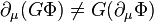
The failure of the derivative to commute with "G" introduces an additional term (in keeping with the product rule) which spoils the invariance of the Lagrangian. In order to rectify this we define a new derivative operator such that the derivative of will again transform identically with

This new "derivative" is called a covariant derivative and takes the form
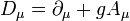
Where g is called the coupling constant – a quantity defining the strength of an interaction. After a simple calculation we can see that the gauge field A(x) must transform as follows

The gauge field is an element of the Lie algebra, and can therefore be expanded as

There are therefore as many gauge fields as there are generators of the Lie algebra.
Finally, we now have a locally gauge invariant Lagrangian

Pauli calls gauge transformation of the first type to the one applied to fields as , while the compensating transformation in  is said to be a gauge transformation of the second type.
The difference between this Lagrangian and the originalglobally gauge-invariant Lagrangian is seen to be theinteraction Lagrangian

This term introduces interactions between the n scalar fields just as a consequence of the demand for local gauge invariance. However, to make this interaction physical and not completely arbitrary, the mediator A(x) needs to propagate in space. That is dealt with in the next section by adding yet another term,  , to the Lagrangian. In the quantized version of the obtained classical field theory, the quanta of the gauge field A(x) are called gauge bosons. The interpretation of the interaction Lagrangian in quantum field theory is of scalar bosons interacting by the exchange of these gauge bosons.
[edit]The Yang–Mills Lagrangian for the gauge field
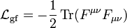
The picture of a classical gauge theory developed in the previous section is almost complete, except for the fact that to define the covariant derivatives D, one needs to know the value of the gauge field  at all space-time points. Instead of manually specifying the values of this field, it can be given as the solution to a field equation. Further requiring that the Lagrangian which generates this field equation is locally gauge invariant as well, one possible form for the gauge field Lagrangian is (conventionally) written as
with
-
![\ F_{\mu \nu} = \frac{1}{ig}[D_\mu, D_\nu]](http://upload.wikimedia.org/wikipedia/en/math/1/3/2/1323cc11c2b9bc772184609ce171e456.png)
and the trace being taken over the vector space of the fields. This is called the Yang–Mills action. Other gauge invariant actions also exist (e.g. nonlinear electrodynamics, Born–Infeld action, Chern–Simons model, theta term etc.).
Note that in this Lagrangian term there is no field whose transformation counterweighs the one of . Invariance of this term under gauge transformations is a particular case of a priori classical (geometrical) symmetry. This symmetry must be restricted in order to perform quantization, the procedure being denominated gauge fixing, but even after restriction, gauge transformations may be possible.[3]
The complete Lagrangian for the gauge theory is now
-

[edit]An example: Electrodynamics
As a simple application of the formalism developed in the previous sections, consider the case ofelectrodynamics, with only the electron field. The bare-bones action which generates the electron field's Dirac equation is

The global symmetry for this system is
-

The gauge group here is U(1), just the phase angle of the field, with a constant θ.
"Local"ising this symmetry implies the replacement of θ by θ(x).
An appropriate covariant derivative is then
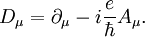
Identifying the "charge" e with the usual electric charge (this is the origin of the usage of the term in gauge theories), and the gauge field A(x) with the four-vector potential of electromagnetic fieldresults in an interaction Lagrangian
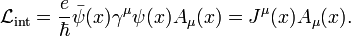
where  is the usual four vector electric current density. The gauge principle is therefore seen to naturally introduce the so-called minimal coupling of the electromagnetic field to the electron field.
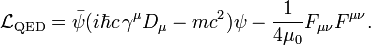
Adding a Lagrangian for the gauge field  in terms of the field strength tensor exactly as in electrodynamics, one obtains the Lagrangian which is used as the starting point in quantum electrodynamics.
- See also: Dirac equation, Maxwell's equations, Quantum electrodynamics
[edit]Mathematical formalism
Gauge theories are usually discussed in the language of differential geometry. Mathematically, agauge is just a choice of a (local) section of some principal bundle. A gauge transformation is just a transformation between two such sections.
Although gauge theory is dominated by the study of connections (primarily because it's mainly studied by high-energy physicists), the idea of a connection is not central to gauge theory in general. In fact, a result in general gauge theory shows that affine representations (i.e. affine modules) of the gauge transformations can be classified as sections of a jet bundle satisfying certain properties. There are representations which transform covariantly pointwise (called by physicists gauge transformations of the first kind), representations which transform as a connection form (called by physicists gauge transformations of the second kind, an affine representation) and other more general representations, such as the B field in BF theory. There are more general nonlinear representations (realizations), but are extremely complicated. Still, nonlinear sigma models transform nonlinearly, so there are applications.
If there is a principal bundle P whose base space is space or spacetime and structure group is a Lie group, then the sections of P form a principal homogeneous space of the group of gauge transformations.
Connections (gauge connection) define this principal bundle, yielding a covariant derivative ∇ in each associated vector bundle. If a local frame is chosen (a local basis of sections), then this covariant derivative is represented by the connection form A, a Lie algebra-valued 1-form which is called the gauge potential in physics. This is evidently not an intrinsic but a frame-dependent quantity. The curvature form F is constructed from a connection form, a Lie algebra-valued 2-formwhich is an intrinsic quantity, by

where d stands for the exterior derivative and  stands for the wedge product. (
 is an element of the vector space spanned by the generators
  , and so the components of do not commute with one another. Hence the wedge product
  does not vanish.)
Infinitesimal gauge transformations form a Lie algebra, which is characterized by a smooth Lie algebra valued scalar, ε. Under such an infinitesimal gauge transformation,
![\delta_\varepsilon \bold{A}=[\varepsilon,\bold{A}]-\mathrm{d}\varepsilon](http://upload.wikimedia.org/wikipedia/en/math/6/d/c/6dc17d6d583f69c95e14a295acfdab9f.png)
where ![[\cdot,\cdot]](http://upload.wikimedia.org/wikipedia/en/math/3/5/8/3587c5df5edf1176ed7afc1f20f5d8a9.png) is the Lie bracket.
is the Lie bracket.
One nice thing is that if  , then
  where D is the covariant derivative

Also,  , which means
  transforms covariantly.
Not all gauge transformations can be generated by infinitesimal gauge transformations in general. An example is when the base manifold is a compact manifold without boundary such that the homotopyclass of mappings from that manifold to the Lie group is nontrivial. See instanton for an example.
The Yang–Mills action is now given by
-
![\frac{1}{4g^2}\int \operatorname{Tr}[*F\wedge F]](http://upload.wikimedia.org/wikipedia/en/math/6/6/c/66c6b841dde36016347a34e90f75b114.png)
where * stands for the Hodge dual and the integral is defined as in differential geometry.
A quantity which is gauge-invariant i.e. invariant under gauge transformations is the Wilson loop, which is defined over any closed path, γ, as follows:

where χ is the character of a complex representation ρ and  represents the path-ordered operator.
[edit]Quantization of gauge theories
Gauge theories may be quantized by specialization of methods which are applicable to any quantum field theory. However, because of the subtleties imposed by the gauge constraints (see section on Mathematical formalism, above) there are many technical problems to be solved which do not arise in other field theories. At the same time, the richer structure of gauge theories allow simplification of some computations: for example Ward identities connect different renormalization constants.
[edit]Methods and aims
The first gauge theory to be quantized was quantum electrodynamics (QED). The first methods developed for this involved gauge fixing and then applying canonical quantization. The Gupta–Bleulermethod was also developed to handle this problem. Non-abelian gauge theories are now handled by a variety of means. Methods for quantization are covered in the article on quantization.
The main point to quantization is to be able to compute quantum amplitudes for various processes allowed by the theory. Technically, they reduce to the computations of certain correlation functions in the vacuum state. This involves a renormalization of the theory.
When the running coupling of the theory is small enough, then all required quantities may be computed in perturbation theory. Quantization schemes intended to simplify such computations (such as canonical quantization) may be called perturbative quantization schemes. At present some of these methods lead to the most precise experimental tests of gauge theories.
However, in most gauge theories, there are many interesting questions which are non-perturbative. Quantization schemes suited to these problems (such as lattice gauge theory) may be called non-perturbative quantization schemes. Precise computations in such schemes often requiresupercomputing, and are therefore less well-developed currently than other schemes.
[edit]Anomalies
Some of the symmetries of the classical theory are then seen not to hold in the quantum theory — a phenomenon called an anomaly. Among the most well known are:
[edit]Pure gauge
A pure gauge is the set of field configurations obtained by a gauge transformation on the null field configuration. So it is a particular "gauge orbit" in the field configuration's space.
In the abelian case, where  , the pure gauge is the set of field configurations
 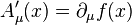 for all f(x).
[edit]See also
[edit]References
[edit]Bibliography
- General readers
- Schumm, Bruce (2004) Deep Down Things. Johns Hopkins University Press. Esp. chpt. 8. A serious attempt by a physicist to explain gauge theory and the Standard Model with little formal mathematics.
- Texts
- Articles
[edit]External links


